Model Confidence: From Ensemble Disagreement to Calibrated Scores

See It in Action

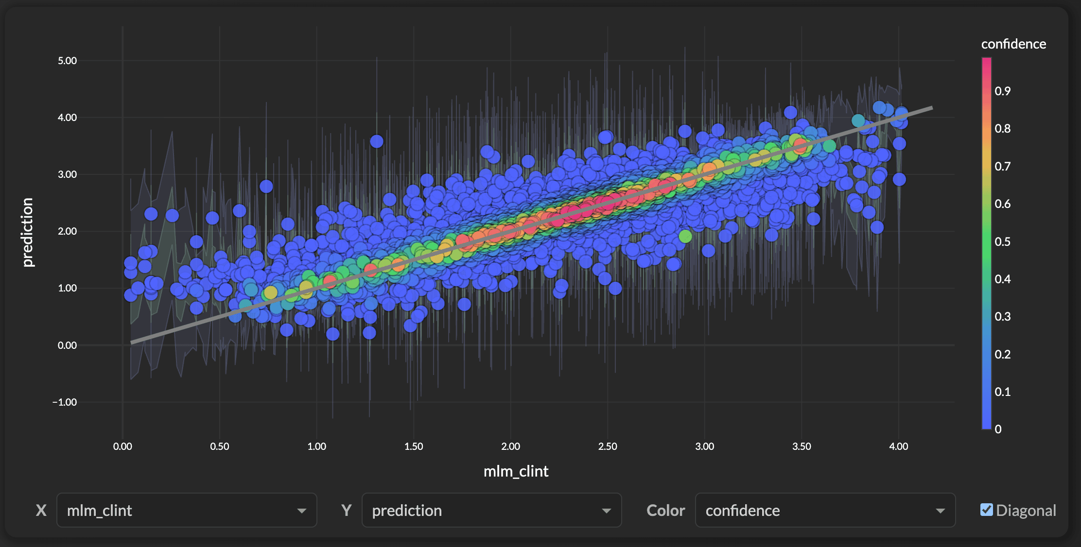
The Confusion Explorer uses these confidence scores to let you filter predictions by certainty and drill down on errors interactively.

A prediction without a confidence score is just a number. In drug discovery, knowing how much to trust a prediction is often more valuable than the prediction itself — it determines whether you synthesize a compound, run an experiment, or move on. In this blog we'll walk through how Workbench approaches model confidence, the trade-offs we've considered, and where we think there's room to improve.

A target vs. prediction scatter from a LogD model on the OpenADMET ExpansionRX challenge test data. Points are colored by confidence — the high confidence points cluster along the diagonal, low confidence (blue) are scattered.

The Core Idea: Ensemble Disagreement

Every Workbench model — whether XGBoost, PyTorch, or ChemProp — is actually a 5-model ensemble trained via cross-validation. Each fold produces a model that saw a slightly different slice of the training data. At inference time, all 5 models make a prediction and we take the average.

The idea behind using ensemble disagreement as an uncertainty signal is well-established in the ML literature (see Lakshminarayanan et al., 2017): when the models disagree, the prediction is less reliable. If all 5 models predict log CLint = 2.4 ± 0.02, we have reason to be confident. If they predict 2.4 ± 0.71, something about that compound is tricky and we should be cautious.

This ensemble standard deviation (prediction_std) is the raw uncertainty signal. It comes directly from the model itself — not from an external surrogate or statistical assumption. In our testing, it correlates strongly with actual prediction error (Spearman r > 0.85 for ChemProp on MLM CLint from the OpenADMET Blind Challenge), though your mileage will vary depending on the dataset and model type.

One implementation note: we apply a soft log-compression to extreme prediction_std outliers (values above the IQR fence get log-scaled) before storing. This is a monotonic transform that preserves ranking — so percentile-rank confidence and conformal intervals are unaffected — but it means reported prediction_std values should be read as "uncertainty scores" rather than literal standard deviations.

The Problem: Raw Std Isn't Calibrated

Ensemble std tells you which predictions to trust more, but the raw numbers don't correspond to meaningful intervals. If std = 0.3, does that mean the true value is within ± 0.3? ± 0.6? There's no guarantee.

This is the classic calibration vs. discrimination trade-off described in Gneiting et al., 2007:

• Discrimination (ranking): Can you tell which predictions are better? Ensemble std tends to do this well.
• Calibration (coverage): Do your 80% intervals actually contain 80% of true values? Raw std alone doesn't guarantee this.

We need both. That's where conformal prediction comes in.

Conformal Calibration

Conformal prediction is a distribution-free framework for turning any uncertainty estimate into calibrated prediction intervals. Originally developed by Vovk et al. and made accessible by Angelopoulos & Bates (2021), the core idea is elegant and the math is straightforward:

1. Compute nonconformity scores on held-out validation data: score = |actual - predicted| / std
2. Find scaling factors: For each confidence level (50%, 68%, 80%, 90%, 95%), find the quantile of scores that achieves the target coverage
3. Build intervals: prediction ± scale_factor × std

The scaling factors are computed once during training and stored as metadata. At inference, building intervals is a simple multiply — no extra models to run.

In practice, this gives us intervals that inherit the ensemble's discrimination (width varies per-compound based on model disagreement) but are calibrated to have correct coverage, an 80% interval should contain ~80% of true values.

Confidence Scores

With calibrated intervals in hand, we compute a confidence score between 0 and 1 for every prediction. The naïve approach is to use ensemble std directly: rank a prediction's std against the cal-set distribution. That works most of the time but has a known failure mode — when the ensemble unanimously agrees on a prediction that's nonetheless wrong, std-based confidence has no way to surface the problem.

This happens most often near censoring boundaries or in dense regions of target space. Solubility is a textbook example: kinetic-sol assays cap at ~-3.5 LogS, producing a large training cluster at -3.5 to -3.7. When the model encounters a chemically similar compound whose true LogS is much lower (say -5.5), all 5 ensemble members tend to converge on the attractor and predict -3.6 anyway — including the one that didn't see the compound during training. The ensemble agreement is genuine but uninformative; the prediction is confidently wrong.

To address this, we use a residual-aware confidence metric. Instead of ranking std directly, we fit a locally adaptive calibrator that maps (prediction, prediction_std) → expected |residual|, then rank the expected residual against the cal-set distribution:

expected_residual = calibrator(prediction, prediction_std)
confidence = 1 - percentile_rank(expected_residual)

The calibrator is fit on the cross-fold validation data, where every compound's residual comes from a model that didn't see it during training. We bin predictions into quantile bins along the prediction axis and fit an IsotonicRegression(std → |residual|) within each bin. At inference this becomes a fast np.interp lookup — no sklearn dependency in production.

This is the standard locally adaptive conformal prediction approach from Lei et al. (2018) applied to the scalar confidence score: instead of treating ensemble disagreement as a constant indicator of uncertainty, we let the data tell us how std actually relates to error in different regions of prediction space.

Interpretation: confidence of 0.7 means "this prediction's expected error is lower than 70% of cal-set predictions." Unlike the naïve std-percentile approach, this is now a probabilistically meaningful statement: among compounds with similar (prediction, std) signatures, roughly 70% will have lower error than this one. Two compounds with identical std but predictions in different regions of target space can now get different confidence scores — which is the right behavior, because std means different things in different regions.

Confidence vs. prediction residual — high-confidence predictions (right) cluster near zero error, while low-confidence predictions (left) show the largest residuals.

A residual-aware metric isn't magic. When good and bad predictions share the same (prediction, std) signature — same prediction, same ensemble agreement — no post-hoc calibrator can distinguish them. In our solubility example, ~96% of compounds with prediction ≈ -3.6 and tight std are correctly predicted; the remaining 4% have true values far from -3.6. The calibrator will assign them all roughly the same moderate-high confidence, because that's what the population-level evidence supports. Distinguishing the unlucky 4% requires either fixing the upstream model bias (e.g., censored-aware training with bounded_loss=True) or adding chemistry-aware applicability-domain features — both of which are orthogonal to the UQ pipeline itself.

Classification Confidence

Everything above applies to regression models — where prediction_std gives us a natural uncertainty signal. But what about classifiers? A classification ensemble doesn't predict a continuous value with a standard deviation; it produces class probabilities. We need a different approach.

The Challenge

For classification, each of the 5 ensemble members outputs a softmax probability distribution over classes. We average those distributions to get the final _proba columns. But how do we turn that into a single confidence score?

Simple approaches like using the maximum predicted probability (max(p)) are tempting but have known issues — Galil et al. (2023) showed that max probability alone is suboptimal for detecting incorrect predictions, especially under distribution shift. It ignores both the shape of the probability distribution and whether the ensemble actually agrees.

VGMU: Variance-Gated Margin Uncertainty

We use VGMU (Variance-Gated Margin Uncertainty), introduced in the Variance-Gated Ensembles paper (2025). The idea is to combine two signals:

• Margin: How much does the ensemble prefer its top class over the runner-up?
• Agreement: Do the 5 models agree on those probabilities, or are they all over the place?

The formula computes a signal-to-noise ratio between the margin and the ensemble disagreement:

\[\text{SNR} = \frac{\bar{p}_1 - \bar{p}_2}{\sigma_1 + \sigma_2 + \epsilon}, \qquad \gamma = 1 - e^{-\text{SNR}}, \qquad C = \gamma \cdot \bar{p}_1\]

where \(\bar{p}_1\) and \(\bar{p}_2\) are the mean probabilities for the top two classes, and \(\sigma_1\) and \(\sigma_2\) are the standard deviations of those probabilities across the 5 ensemble members.

This gives us nice behavior across the spectrum:

• Ensemble agrees with clear margin → high SNR → gamma ≈ 1 → confidence ≈ p_top1
• Ensemble disagrees or margin is thin → low SNR → gamma ≈ 0 → confidence ≈ 0
• Uniform probabilities (model can't distinguish classes) → margin = 0, confidence = 0

Isotonic Calibration

Just like raw ensemble std needs conformal calibration for regression, raw VGMU scores need calibration for classification. We use isotonic regression — a standard technique that fits a monotonically non-decreasing mapping from raw confidence to empirical accuracy on the validation set.

During training, we compute VGMU scores for all validation predictions and fit an isotonic regression mapping raw_confidence → P(correct). The fitted mapping is stored as a simple piecewise-linear function (just two arrays of thresholds) that can be applied with np.interp at inference time — no sklearn dependency needed in production.

After calibration, a confidence of 0.85 means that among validation predictions with similar VGMU scores, about 85% were correctly classified. This gives the score a direct probabilistic interpretation.

Training output

During training, classification models now print calibration diagnostics showing how raw confidence maps to actual accuracy across bins:

==================================================
Calibrating Classification Confidence (VGMU)
==================================================
  Validation samples: 2451
  Overall accuracy: 0.847
  Raw confidence  - mean: 0.621, std: 0.284
  Calibrated conf - mean: 0.847, std: 0.128
  Bin 1: n=  490, accuracy=0.639, calibrated_conf=0.654
  Bin 2: n=  490, accuracy=0.794, calibrated_conf=0.805
  Bin 3: n=  490, accuracy=0.871, calibrated_conf=0.873
  Bin 4: n=  491, accuracy=0.924, calibrated_conf=0.922
  Bin 5: n=  490, accuracy=0.998, calibrated_conf=0.982

This lets you verify that the calibration is working — accuracy should increase monotonically across bins, and calibrated confidence should track accuracy closely.

Unified Across Frameworks

One design goal we're happy with: the same UQ pipeline runs for all three model types. Each framework trains its ensemble differently, but the uncertainty signal and calibration pipeline are unified — conformal scaling for regression, VGMU + isotonic calibration for classification.

Framework	Ensemble	Regression Confidence	Classification Confidence
XGBoost	5-fold CV	Ensemble std + conformal scaling	VGMU + isotonic calibration
PyTorch	5-fold CV	Ensemble std + conformal scaling	VGMU + isotonic calibration
ChemProp	5-fold CV	Ensemble std + conformal scaling	VGMU + isotonic calibration

This consistency means confidence scores have the same interpretation across frameworks, which simplifies things when comparing models on the same dataset.

What Confidence Doesn't Tell You

We want to be upfront about the limitations. Confidence reflects how much the ensemble models agree — but agreement doesn't guarantee correctness. All 5 models can confidently agree on the wrong answer, especially for compounds that are structurally far from the training data.

• High confidence ≠ correct prediction. It means the models agree, not that they're right. This is a fundamental limitation of ensemble-based UQ noted by Ovadia et al., 2019.
• Novel chemistry may get falsely high confidence if it happens to fall in a region where the models extrapolate consistently.
• Confidence is relative to the training set. A confidence of 0.9 on a kinase solubility model doesn't transfer to a PROTAC dataset.
• Conformal coverage assumes exchangeability. The guarantee holds when test data comes from the same distribution as calibration data. For out-of-distribution compounds, coverage may degrade.
• Training-exposure bias in calibration. Calibration prediction_std is computed by running all 5 ensemble members on the full training set, so every row was seen by 4 of the 5 models during training. Truly novel molecules (seen by 0 of 5) will tend to produce larger stds than the calibration distribution captures, which can make confidence skew optimistic-then-low on out-of-distribution chemistry. The residual-aware calibrator helps here by anchoring confidence to historical errors rather than raw std — but it doesn't eliminate the bias. Workbench now defaults to scaffold-based cross-validation splits (Bemis-Murcko) for any dataset with a SMILES column, which makes confidence calibration reflect scaffold-hopping performance rather than same-scaffold interpolation. For stricter "novel chemistry" evaluation, set split_strategy="butina" (Morgan-fingerprint clustering).
• Indistinguishable populations within a calibration bin. When a chunk of compounds shares the same (prediction, std) signature but a subset are wrong (e.g. censored-data attractors in solubility), the residual-aware metric assigns them all roughly the same confidence — population-correct, but unable to flag individual unlucky misses. Addressing this requires either upstream model fixes (censored-aware training) or chemistry-aware applicability-domain features, neither of which is part of the confidence pipeline itself.

For truly out-of-distribution detection, we'd recommend pairing confidence with applicability domain analysis (e.g., feature-space proximity to training data). This is something we're actively exploring for future Workbench releases.

Summary

Here's how Workbench approaches model confidence today:

Regression models:

1. Ensemble disagreement — Building on Lakshminarayanan et al., the 5-fold CV ensemble provides prediction_std as the raw uncertainty signal
2. Conformal calibration — Following Angelopoulos & Bates, we scale std into prediction intervals with target coverage (80% CI → ~80% coverage)
3. Residual-aware confidence — Following Lei et al. (2018), a locally adaptive calibrator maps (prediction, std) → expected |residual|, then ranks the expected residual against the cal-set distribution. This surfaces the failure mode where ensemble disagreement is artificially low in dense regions of target space (e.g. near censoring boundaries)

Classification models:

1. Ensemble probabilities — Each of the 5 models outputs class probabilities; we average them and also track per-model disagreement
2. VGMU scoring — Following Gillis et al. (2025), we combine the probability margin between top classes with ensemble disagreement via a signal-to-noise ratio
3. Isotonic calibration — Maps raw VGMU scores to P(correct) using isotonic regression on validation data, giving confidence a direct probabilistic interpretation

Both approaches share the same philosophy: leverage the ensemble's own disagreement as the uncertainty signal, then calibrate it against held-out data so the numbers are meaningful. We're excited about this unified framework and looking forward to incorporating applicability domain methods and testing on a wider range of datasets.

References

• Lakshminarayanan et al., "Simple and Scalable Predictive Uncertainty Estimation using Deep Ensembles" (2017) — Foundational work on using ensemble disagreement for uncertainty
• Vovk et al., "Algorithmic Learning in a Random World" — Foundational text on conformal prediction
• Angelopoulos & Bates, "Conformal Prediction: A Gentle Introduction" (2021) — Accessible introduction to conformal methods
• Lei et al., "Distribution-Free Predictive Inference for Regression" (2018) — Locally adaptive conformal prediction; basis for the residual-aware confidence calibrator
• Gneiting et al., "Probabilistic Forecasts, Calibration and Sharpness" (2007) — Calibration vs. discrimination framework
• Ovadia et al., "Can You Trust Your Model's Uncertainty?" (2019) — Analysis of ensemble UQ under dataset shift
• Gillis et al., "Variance-Gated Ensembles: An Epistemic-Aware Framework" (2025) — VGMU approach for combining margin and ensemble variance in classification
• Galil et al., "What Can We Learn From The Selective Prediction And Uncertainty Estimation Performance Of 523 Imagenet Classifiers?" (2023) — Analysis showing entropy-based measures outperform max probability for failure detection
• Wimmer et al., "Quantifying Aleatoric and Epistemic Uncertainty in Machine Learning: Are Conditional Entropy and Mutual Information Appropriate Measures?" (2023) — Caveats on entropy decomposition for small ensembles
• OpenADMET Blind Challenge — ExpansionRx MLM CLint dataset used for examples in this blog

Questions?

The SuperCowPowers team is happy to answer any questions you may have about AWS and Workbench. Please contact us at workbench@supercowpowers.com or on chat us up on Discord