Hyperparameter Optimization (HPO)

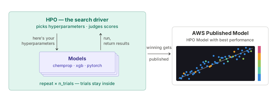
HPO wraps normal model creation. The search driver hands a set of hyperparameters to the same training code that publishes your models, gets a score back, and repeats — all inside a single training job. Trials are ephemeral: they never create Workbench models or endpoints, so a searched model looks like any other model.

Available for ChemProp, XGBoost, and PyTorch, regression only.

Running a search

An otherwise normal to_model() call plus an hpo block:

from workbench.api import FeatureSet, ModelType, ModelFramework

fs = FeatureSet("aqsol_features")

model = fs.to_model(
    name="sol-xgb-hpo",
    model_type=ModelType.UQ_REGRESSOR,
    model_framework=ModelFramework.XGBOOST,
    target_column="solubility",
    feature_list=fs.feature_columns,
    description="Solubility regression (hyperparameter-searched)",
    tags=["solubility", "hpo"],
    hyperparameters={"uq_version": "v1", "hpo": {"n_trials": 250}},
)

The winning configuration becomes the model's hyperparameters, so the published model is deployed and used exactly like any other.

The `hpo` block

key	default	what it does
`n_trials`	`60`	search budget — how many configurations to try
`search_space`	all groups	which knob groups to search — see below
`metric`	`cv_mae`	objective: `cv_mae` (out-of-fold) or `holdout_mae`
`rerank_top_k`	`5`	finalists re-scored in the second stage (`0` disables it)
`backend`	`auto`	`optuna` (serial) or `ray` (parallel, needs a GPU box)
`max_parallel`	`1`	concurrent trials (Ray only)
`n_folds`	model's `n_folds`	ensemble size per trial — for cheap validation runs only

The searched knobs differ per framework, and a model knows its own — hpo_search_space() dispatches on the model's framework and returns one row per knob, carrying its range and where it sits untuned. A space is judgeable without running anything:

model.hpo_search_space()           # every knob for this model's framework

Three columns are pinned — knob, default, dist — and everything specific to the distribution rides in a spec JSON object, so knobs of different kinds share one table without leaving holes:

knob	default	dist	spec
`max_depth`	7	int	`{"low": 3, "high": 16, "step": 1}`
`learning_rate`	0.05	float	`{"low": 0.003, "high": 0.3, "log": true}`
`ffn_hidden_dim`	1800	choice	`{"options": [300, 600, "1024-256-64", ...]}`

json.loads the spec cell to read it. This is always the framework's full space.

To search only part of it, set hpo["search_space"] to a group name or a +-joined combination. basic is capacity everywhere; the second group differs because the frameworks' second lever does:

framework	groups
ChemProp, PyTorch	`basic` + `optimizer` (learning rate, batch size)
XGBoost	`basic` + `reg` (sampling and penalty terms)

So hpo={"search_space": "basic"} spends the whole budget on architecture — useful when you already trust your optimizer settings.

Your own ranges and defaults

A default is just a hyperparameter. Set a knob normally alongside the hpo block and it becomes the baseline the search has to beat — and the value used for any knob outside the searched groups:

hyperparameters={"uq_version": "v1", "max_lr": 3e-3, "depth": 4, "hpo": {"n_trials": 60}}

A range needs a SearchSpace. Start from the shipped space, change the knobs you have an opinion about, and hand the result to hpo["search_space"]:

from workbench.training.hpo_harness import SearchSpace, IntRange, FloatRange

space = SearchSpace("xgboost")                              # or "chemprop" / "pytorch"
space["max_depth"] = IntRange(4, 8, default=6)              # your ceiling, not ours
space["learning_rate"] = FloatRange(0.02, 0.06, log=True)
del space["gamma"]                                          # not worth trials on this data

fs.to_model(..., hyperparameters={"uq_version": "v1",
                                  "hpo": {"n_trials": 60, "search_space": space.to_dict()}})

SearchSpace is a dict subclass, so ordinary space[knob] = ... and del are the whole editing API. .subset("basic") narrows to a group, and .to_frame() gives the same table hpo_search_space() returns, for checking your work.

What you pass is the whole space — a one-knob dict searches one knob, it does not patch ours. That is what makes space.to_dict() the natural starting point.

to_dict() emits plain JSON, which is also what hpo["search_space"] accepts directly if you would rather write it out:

hpo={"search_space": {"max_depth": {"dist": "int", "low": 4, "high": 8, "default": 6},
                      "learning_rate": {"dist": "float", "low": 0.02, "high": 0.06, "log": True}}}

dist is required — "int", "float", or "choice" — and default is optional, falling back to the framework's. Bad spaces fail immediately rather than on trial 40: an inverted range, a log scale starting at zero, or an empty option list all raise at construction.

Selection is two-stage

A search reports the minimum over many noisy estimates, so its winning value is optimistically biased — the winner may simply have drawn the luckiest evaluation. Workbench therefore treats the search as a shortlist, not a decision:

Search — sample the space, and prune configurations that are already off the pace.
Re-rank — re-score the top finalists and your own untuned hyperparameters on fresh trainings, then publish whichever wins.

Carrying your own hyperparameters through the second stage is what bounds the downside: a search that finds nothing real loses to them, and your original settings get published unchanged. Ties go to your settings.

That makes a baseline win a legitimate outcome rather than a failed run — it means the search spent the compute and confirmed your existing configuration.

Reading the results

One call resolves the training job's artifacts — no hunting for S3 paths or CloudWatch logs. A None return doubles as the "was this model searched?" check.

results = model.hpo_results()

{'metric': 'cv_mae',
 'trial_counts': {'attempted': 100, 'completed': 34, 'pruned': 66, 'failed': 0},
 'best_config': {'layers': '128-64',
                 'dropout': 0.25,
                 'learning_rate': 0.0002846282635669909,
                 'weight_decay': 0.0014020994043985207,
                 'batch_size': 128},
 'best_value': 0.5106314063072205,
 'baseline_value': 0.5450914978981019,
 ...}

best_config is what shipped. These are the model's hyperparameters now — you can hand the dict straight to another to_model() call to train a sibling on different data:

fs.to_model(name="pxr-reg-pytorch-v2", ..., hyperparameters={"uq_version": "v1", **results["best_config"]})

best_value vs baseline_value is the headline. Both are metric (here cv_mae, lower is better) on the same basis, so their difference is the margin the publish decision turned on — quote this pair:

gain = 100 * (results["baseline_value"] - results["best_value"]) / results["baseline_value"]
print(f"{results['metric']}: {results['best_value']:.4f} vs {results['baseline_value']:.4f} baseline ({gain:+.1f}%)")
# cv_mae: 0.5106 vs 0.5451 baseline (+6.3%)

trial_counts tells you whether the budget was spent well. A high pruned count is the pruner working as intended — those trials were stopped early once they fell off the pace, so completed is what ran to term. Any failed at all is worth a look at the training log.

The trials frame

trials = results["trials"]      # one row per trial, plus a `baseline` row

number	value	completed	kind	hyperparameters
0	0.516991	True	trial	`{"layers": "256-128", ...}`
1	0.530321	False	trial	`{"layers": "512-256-64", ...}`

hyperparameters is a JSON object of every searched knob and the value it actually trained at, so each row is complete and NaN-free — expand it with json.loads to get one column per knob:

import json
import pandas as pd

df = pd.DataFrame([json.loads(h) for h in trials["hyperparameters"]])
df["value"] = trials["value"].values
df.nsmallest(5, "value")                        # the finalists the re-rank scored
df.groupby("layers")["value"].agg(["count", "mean", "min"])

completed=False marks a pruned trial: its value is the last score before it was stopped, so it is a lower bound, not a finished result. The single kind="baseline" row is your own untuned config scored on the same basis as the trials — it is the reference line any plot of the search needs, and results["rerank"] holds the finalists' re-scores if you want the second stage's own numbers.

Which knobs mattered

hpo_importance() answers that from the search's own trials — useful for deciding where to spend the next budget, or whether a knob earns its place in the space at all:

model.hpo_importance()          # None if the model was not searched

knob	importance	effect	best
`max_lr`	0.51	7.9%	0.0043
`batch_size`	0.37	7.8%	512
`hidden_dim`	0.07	2.4%	100
`depth`	0.02	0.5%	5

Read the two numbers together. importance is a share and always sums to 1, so in a search where nothing mattered something still looks important. effect is the absolute read — how far the objective moves across that knob's range, as a percentage of the objective. A knob is worth tuning only when both are high; depth above holds a real share of very little. best is where the objective bottoms out with the other knobs averaged out, which is meaningless when effect is small.

How it's computed. The trials are the dataset — knob values in, objective out — and a random forest is fit to that response surface. importance is the forest's split-based importance; effect and best come from a partial-dependence sweep, which pins one knob across its range while averaging over the others.

That averaging is the point. A search is not a designed experiment: the sampler concentrates trials where it thinks the optimum is, so a knob's raw group means are confounded with whatever else it happened to be exploring at the time. Marginalizing the other knobs out is what makes one knob's effect readable on its own. A forest suits the job because the response is small-N, riddled with interactions, and often non-monotone — a learning rate with an interior optimum has a rank correlation near zero, which would read as "irrelevant" to a simpler measure. It is also the field standard: fANOVA, what Optuna reports, is random-forest-based too.

Two limits worth knowing. Split-based importance is biased toward knobs with more distinct values, which is part of why effect is there as a differently-biased second opinion. And partial dependence extrapolates — where the sampler correlated two knobs, the sweep asks the forest about combinations the search never actually tried. These are observational estimates over a few dozen trials, not a controlled ablation, so treat the ordering as directional.

How it fits together

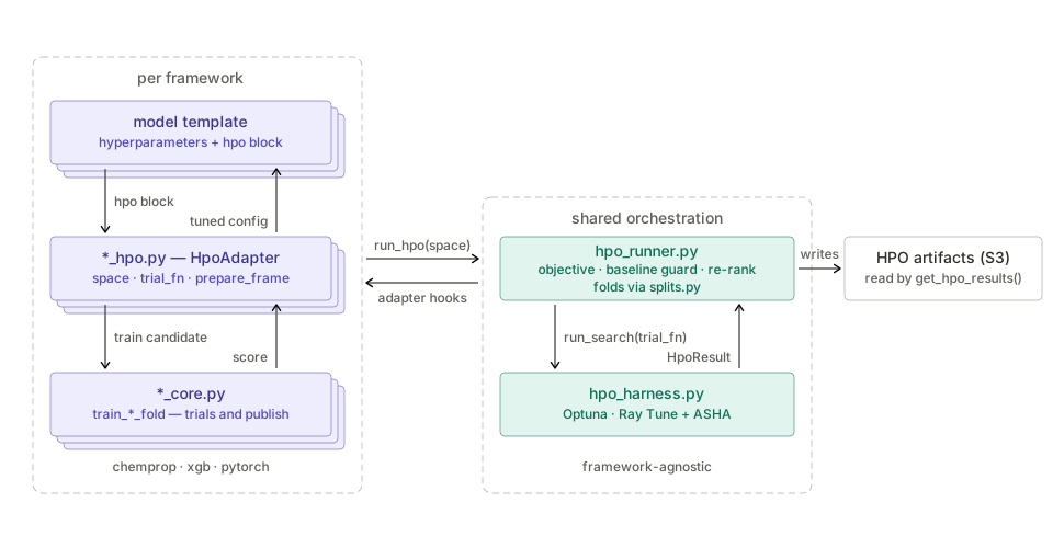
Everything on the left is per-framework — one model template, one adapter, and one fold trainer for each of ChemProp, XGBoost, and PyTorch. Everything on the right is shared and knows nothing about any framework.

A template hands its hpo block to its adapter, which calls run_hpo. From there control inverts: the runner drives the search and calls back into the adapter for the framework-specific parts — the search space, how to train and score one candidate, and how a winning config merges back into the hyperparameters. That boundary is why all three frameworks produce identical artifacts and hpo_results() needs no per-framework logic.

The detail that makes a search result mean anything is at the bottom left: a trial and the final published model train through the same train_*_fold function. A configuration is therefore scored in exactly the regime it ships in.

What to expect

Temper expectations. Framework defaults are a strong baseline and often win on small datasets, and the literature finds ChemProp HPO is roughly a coin flip against defaults there. Measured on our own data, HPO improved in-distribution cross-validation but lost to stock defaults on a held-out analog series — gains on cross-validation do not imply gains on a new chemical series.

By default the objective is cv_mae, scored out-of-fold on the training rows. Rows designated through validation_ids are held out of training and out of the search, so they remain an honest benchmark. Opt into tuning toward them with hpo={"metric": "holdout_mae"} only when that set exists to be tuned against — doing so makes its own final score optimistic.

Questions?

The SuperCowPowers team is happy to answer any questions you may have about AWS® and Workbench.

Support: workbench@supercowpowers.com
Discord: Join us on Discord
Website: supercowpowers.com